Road Lighting Simulation with DIALux EVO

If a lighting plan looks perfect on paper but fails on-site, it wasn’t a design — it was a guess.
This article is written by Sunlurio engineers and lighting consultants with over a decade of project experience. It explains how real engineers use DIALux EVO to design road lighting that passes audits, satisfies both drivers and pedestrians, survives dust and salt, and still meets the energy budget. No screenshots-for-show — only practical methods you can defend in a review meeting.

This guide applies to EN13201-based designs for highways, urban streets, roundabouts, pedestrian routes, and mixed-traffic zones.

1) Why This Guide (and What Others Miss)

Most “how-to” articles stop at menu clicks or paste EN13201 tables. Real projects fail elsewhere — for example:

• Wrong pavement reflection table (R-table) causing low luminance;
• Maintenance Factor (MF) guessed instead of calculated;
• Observer settings missing, making luminance results unreliable;
• Optics chosen by wattage instead of intensity distribution;
• TI (glare) passed in one variant but fails after a small tilt change;
• kWh/km looks good on paper but ignores dimming schedule or cleaning frequency.

Sunlurio insight: A defensible design must be reproducible — explainable, recalculable, and verifiable by auditors.

2) Standards and When to Use Each Metric

According to EN13201, road lighting classes are divided into three main groups:

• M-classes (motorized roads): design by luminance (Lav, Uo, Ul, TI, SR). Used when drivers need to see objects against the road background.
• C-classes (conflict areas): design by illuminance (Eav, Uo, TI). Used for junctions, roundabouts, toll plazas, and bus terminals with mixed traffic.
• P-classes (pedestrian/cycle paths): horizontal Eav/Emin, and when safety and recognition are key, also vertical Ev,min and semi-cylindrical Esc,min.

Field note: For borderline collector roads with both cars and pedestrians, use a dual-grid check — luminance on the carriageway and vertical illuminance on sidewalks. This avoids the classic “numbers pass but faces don’t” issue.

3) Inputs to Freeze Before You Start Modeling

Before launching DIALux EVO, freeze all functional, geometrical, and operational inputs. If they’re uncertain, every result downstream is meaningless.

3.1 Functional & Environmental Parameters

• Target lighting class (M/C/P) and local standards (EN13201, JKR, MoW, BS codes, etc.);
• Design speed and lane function (main road, feeder, local);
• Curfew or dimming strategy (for late-night energy saving);
• Ambient brightness category (A–D) — affects class selection;
• Glare sensitivity (especially near residential or school zones).

3.2 Geometry & Surface Conditions

• Define lanes, width, medians, sidewalks, verge, setback, and overhang;
• Document tolerances (±50–100 mm) — small errors can break TI limits;
• Select the correct R-table: dense asphalt ≠ porous asphalt ≠ concrete;
• Run sensitivity checks — compare Lav/Uo under two plausible R-tables.

3.3 Operational & Power Settings

• Environmental category (urban clean / dusty / coastal) → affects MF;
• Feeder limit (max kW/km), CMS or standalone driver control;
• Dimming schedule — ideally 3–4 stages (e.g., 100% / 70% / 50% / 30%).

Professional tip: Always include an Assumption Register on the first page of your report — MF, R-table, cleaning schedule, dimming strategy, and ambient conditions.

4) Maintenance Factor (MF) — Build It, Don’t Guess

MF defines whether your lighting stays compliant over time or just at installation. It’s the difference between “energy saving” and “non-compliance.”

MF = LLMF × LSF × LMF × RSMF

• LLMF: Lumen Maintenance Factor from LM-80/TM-21 test curves at actual operating temperature.
• LSF: Lamp Survival Factor — usually 1.0 for LEDs, but confirm with surge and ingress data.
• LMF: Luminaire Dirt Factor — depends on environment and cleaning cycle (urban 0.92–0.95, coastal 0.80–0.88).
• RSMF: Road Surface Maintenance Factor — typically 0.97–1.00.

Recommended presets: Urban clean (annual wash): MF = 0.84–0.86; Coastal/dusty (biennial wash): MF = 0.75–0.82.

Tip: Set MF before running calculations in DIALux. This ensures that your results reflect maintained luminance — not new-lamp brightness.

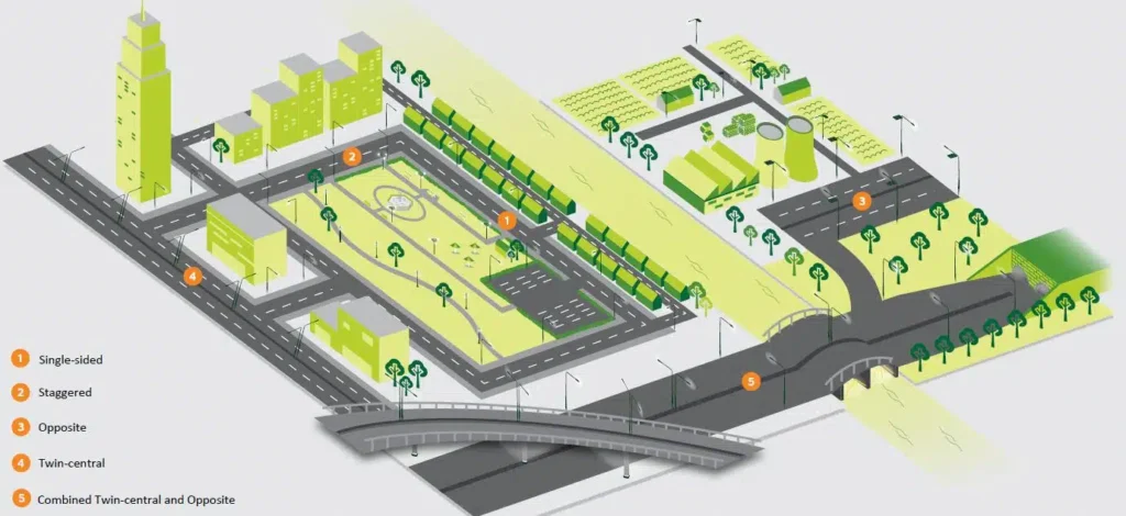
5) Arrangement Matrix by Width/Height Ratio (W/H)

The right pole arrangement defines both uniformity and cost efficiency. Below is a quick reference matrix:

W/H	Arrangement	Advantages	Risks / Fixes
W ≤ H	Single-sided	Good guidance, easy maintenance	Far side dark → wider optic, +1 m height, overhang 0.6–1.0 m
H < W ≤ 1.5H	Staggered	Material efficient	“Zebra effect” → limit tilt, try opposite if Ul < 0.60
W ≥ 1.5H	Opposite	Strong lateral uniformity	Low height glare → raise to 10–12 m or use tighter optic
Dual carriageway with wide median	Twin-central	Fewer columns, clean verge	Maintenance near fast lane → plan closures in O&M

Starting heuristics: S ≈ 3.0–4.2 × H for M3–M5 classes; tilt 0–3°; overhang 0.5–1.0 m. Always choose optics first, tilt last.

Field note: In tropical regions (e.g., Malaysia, Ghana), single-sided layouts often fail on wide roads (>1.2H). Always compare single vs. staggered in DIALux and check Ul ≥0.6.

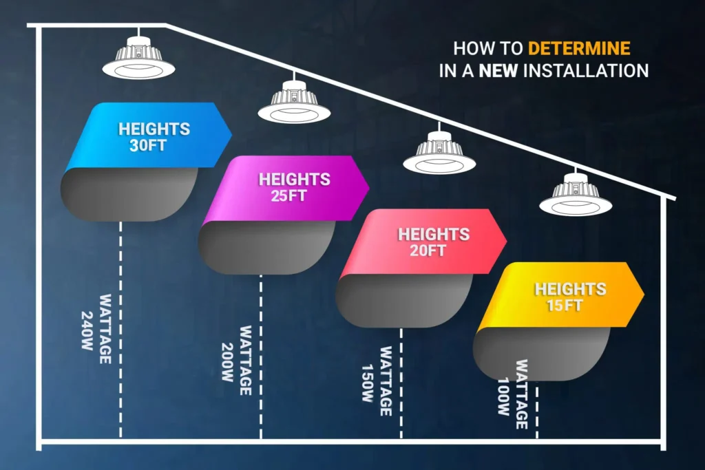
6) Optics, CCT, CRI, and Glare Control (TI)

Optics define perception, not just brightness. Always design from distribution, not wattage.

6.1 Optic Selection Method (Not “Pick a Wattage”)

1. Derive required luminous intensity around observer direction from Lav/Uo/Ul targets.
2. Map manufacturer optics (T2/T3/T4 families) to your W/H and setback — short throw for single-sided, wider for opposite/twin-central.
3. Simulate two optics with the same lumens, compare TI and far-side luminance before touching tilt.

6.2 TI Control Ladder

1. Tilt 0–1° + anti-glare shield;
2. +1 m mounting height (fastest improvement);
3. Change optic to reduce 70–85° intensity;
4. Lower flux + tighter spacing (last resort due to energy cost).

6.3 Color & Visibility

• Arterials: 4000 K, CRI ≥70; Residential/P zones: 3000 K for lower perceived glare;
• Where facial recognition or CCTV is important, ensure vertical Ev ≥2.5 lx and Esc ≥1.5 lx, CRI ≥80.

Lesson learned: In humid climates, high-CCT (5000K) attracts insects and dust, degrading optics and increasing TI. A balanced 3500–4000K works best for long-term stability.

7) DIALux EVO Workflow — What Auditors Expect

7.1 Project Setup

• Use EN13201 mode with proper units and observer settings (speed, height, position);
• Assign correct R-table for each road, enable “wet-road” if required.

7.2 Calculation Grids

• M-class: luminance grid on observer line; verify eye height 1.5 m and distance;
• C/P: horizontal grid; add vertical and semi-cyl grids for pedestrian recognition.

7.3 Luminaires & MF

• Import ULD/IES; set MF now; lock dimming curve candidates (100/70/50/30%).

7.4 Arrangement & Optimization

• Seed: H=9–10 m, S=34–40 m for urban M4; tilt 0°; overhang 0.8 m;
• Run auto-optimization; treat results as a guide, not gospel. Manually fine-tune TI, Uo, Ul.

7.5 Energy Accounting

• Export W/m and kWh/km/year with actual dimming schedule. Always quote the schedule beside the number.

8) From Numbers to Decisions — The Variant Scoring Model

Criterion	Weight	Variant A	Variant B	Notes
Compliance	Gate	Pass	Pass	All targets met
Uo/Ul Margin	25%	0.04/0.03	0.02/0.01	Headroom for aging/re-paving
TI Margin	20%	–3% below limit	–0.5% below	Better rainy-night comfort
Energy (kWh/km/yr)	25%	–12%	–8%	With 100/70/50/30% dimming
CAPEX	20%	–5%	Baseline	Fewer poles but higher height
O&M Risk	10%	Low	Medium	Access near fast lane

Transparent scoring builds client trust — even if they choose a higher-energy option for easier maintenance.

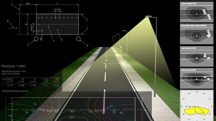
9) Worked Example A — Urban M4 (Single-Sided, 7 m Width)

• Targets: Lav ≥0.75 cd/m², Uo ≥0.40, Ul ≥0.60, TI ≤15%;
• Assumptions: Dense asphalt R-table, MF=0.80, 4000K, CRI ≥70.

9.1 Seed

• H=8 m; S=30 m; overhang 0.8 m; tilt 0°; optic T3; 6,500 lm maintained flux.

9.2 Iteration Logic

• Low Lav → +10% flux or –2 m spacing;
• Weak Uo (far side dark) → wider optic or +1 m height;
• Weak Ul → keep single-sided; adjust S by +2 m; try narrower optic;
• High TI → reduce tilt, +1 m height, or shielded variant.

9.3 Converged Result

• H=9 m; S=36–40 m; 40–55 W driver bin;
• Lav ≈0.80 cd/m²; Uo≥0.42; Ul≥0.62; TI≤15%;
• 1.2–1.5 kW/km full load; 50% dimming after midnight → 35–45% energy savings.

10) Worked Example B — C2 Roundabout (Illuminance-Based)

• Targets: Eav ≥20 lx, Uo ≥0.4, TI ≤15%;
• Tips: Position masts before entries to light conflict points; use symmetric or batwing optics; minimal tilt to reduce glare for exiting drivers.

11) Worked Example C — P3 Sidewalk & Cycle Track (Facial Recognition)

• Targets: Eav ≥7.5 lx, Emin ≥1.5 lx, Uo ≥0.25; Ev,min 2.5 lx; Esc,min 1.5 lx at 1.5 m height.
• Method: Add vertical & semi-cyl grids along path; compare 3000K vs 4000K; CRI ≥70 (≥80 for CCTV areas).

12) Multi-Profile in One DIALux File (and Why It Matters)

• Create separate “roads” for M, C, and P — each with unique grids and reports;
• Use one luminaire family for consistent maintenance, varying optics/wattage;
• Compare variants: 4000K all vs. 3000K for P-zones.

13) Energy & Controls — Numbers Clients Believe

• Always quote kWh/km/year with the dimming schedule beside it (e.g., 100% 18:00–22:00, 70% 22:00–24:00, 50% 00:00–05:00, 70% 05:00–06:00).
• Show sensitivity: if curfew extends to 30%, what happens to Uo and TI? Some optics lose uniformity at low flux.

14) QA & Sign-Off Checklist (Use It in Review Meetings)

• MF basis (LLMF curve + cleaning policy);
• R-table source and sensitivity check;
• Observer settings on first page of M-report;
• Full grid coverage, no clipping at intersections;
• TI verified for wet-road condition (if specified);
• Vertical/semi-cyl grids where recognition is required;
• Dimming schedule printed next to kWh/km/yr;
• BoQ = final H/S/optic/tilt (no seed artifacts).

15) Common Failure Modes (and Fast Remedies)

• “Numbers pass, site feels harsh” → lower tilt; use 3000 K near residences; check TI margin on downhill approaches.
• “Uniformity fine in calc, patchy after resurfacing” → wrong R-table; keep Uo margin ≥0.03.
• “Optimizer loves spacing I can’t build” → lock spacing to pole modules (6 m multiples).
• “Wet-road glare complaints” → re-run wet R-table; limit high-angle intensity; try shielded optic.

16) Deliverables That Withstand Peer Review

• Plan view with IDs, H/S, overhang, tilt, optic code, CCT;
• Compliance tables (Lav/Uo/Ul/TI/SR or Eav/Uo/Ev/Esc);
• Energy page: W/m and kWh/km/yr + printed dimming schedule;
• BoQ: poles, brackets, luminaires, drivers/CMS;
• Assumption register: MF, R-table, environment, access policy.

17) Quick Reference (Pin This Near Your Monitor)

• Single-sided: W ≤ H; start S=3.6×H; far-side → wider optic or +H;
• Staggered: H < W ≤ 1.5H; watch Ul; don’t exceed 3° tilt;
• Opposite: W ≥ 1.5H; use tighter optic to limit TI;
• M4 targets: Lav 0.75, Uo 0.40, Ul 0.60, TI ≤ 15%;
• P3 targets: Eav 7.5 lx, Emin 1.5 lx; Ev 2.5 lx & Esc 1.5 lx if needed.

18) Appendix — Fast Start Template (Copy to Your SOP)

1. Create project → EN13201 mode → units;
2. Road 1 (M): widths, R-table → luminance grid (observer 1.5 m);
3. Import ULD/IES → MF=0.80 → H=9 m, S=36 m seed;
4. Run → adjust optic/tilt/H/S until Lav/Uo/Ul/TI pass with margin;
5. Road 2 (C): junction → horizontal grid → verify Eav/Uo/TI;
6. Road 3 (P): sidewalk/cycle → vertical & semi-cyl grids at 1.5 m;
7. Build Variants: single vs opposite; optic A vs B; 4000 K vs 3000 K;
8. Add dimming scenes → export kWh/km/yr (print schedule);
9. Generate report + BoQ + assumptions register.

19) People Also Ask (Straight Answers)

Q1. Why do my TI results change after a tiny tilt?

Because glare depends on luminous intensity near observer direction (≈70–85°). A 1–2° tilt can push peaks into the danger zone. Fix with lower tilt or a different optic — not just lower wattage.

Q2. Is 5000 K “brighter” than 4000 K?

Photopically only slightly. But it increases glare and discomfort. For mixed or residential areas, 3000–4000 K is safer and more pleasant.

Q3. Can I trust auto-optimization to set spacing?

Use it to locate feasible ranges, not final spacing. Manually adjust for constructability (pole modules), glare control, and real maintenance access.

20) Author

Written by senior lighting engineers delivering M/C/P-class designs across highways, ports, and townships since 2010. If you need a verified DIALux EVO file with your actual geometry, IES data, and compliance tables, contact Sunlurio Technical Center — we deliver reports that pass audits, not just look pretty.